Multiple Criteria Evaluation in Dinamica EGO
What will you learn?
- MCE for urban and regional planning.
Multiple Criteria Evaluation (MCE) is a method often used for environmental impact assessments or urban and regional planning. In this exercise you will apply MCE to identify areas that are favorable to develop a new town in Northern Mato Grosso – an Amazonian frontier region –, mitigating at the same time possible environmental impacts from urban settlement. Again, we confront two points of views, one from developers and another from conservationists. A way to solve this question is to list all criteria that favor the location of a future urban site and the ones that constrain or impede it.
In this problem, we have two types of criteria, the ones that constrain our analysis only to specific areas, thus they are Boolean, either 1 or 0, and the others that assign a degree of suitability for a site depending on its biophysical and infrastructure attributes.
Our criteria are:
- Distance to main roads < 15 kilometers.
- Driving distance to neighboring towns < 30 minutes
- At least 10 km away from existing towns.
- At least 1000 meters away from flooded plains (Malaria is endemic in the region)
- In addition, we need to consider that not all land is available. We don’t want to encourage more deforestation in the region, thus we need to use only land that is deforested or abandoned. Also existing urban areas, rivers and flooded plains must be excluded.
- At least areas larger than 1000 hectares.
- Average slope < 0.5 degrees.
First step: Finding unconstrained areas
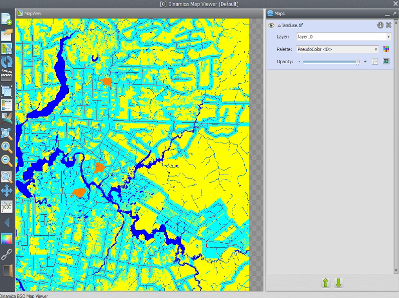
The land use map has the following classes:
| Id | Land use |
|---|---|
| 0 | Flooded plains |
| 1 | Small Rivers |
| 2 | Pasture |
| 3 | Regrowth |
| 4 | Forest Remnant |
| 5 | Urban |
| 6 | Roads |
Load \lesson4\originals\landuse.tif it on the Map Viewer and change the Current color palette to “mt”.
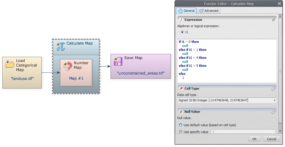
Let's start developing the model. Place Load Categorical Map on the sketch and open the file \lesson4\original\landuse.tif. Now place Calculate Map and Number Map within it. Enter “1” in Map Number in Number Map. Now place Save Map and enter unconstrained_areas.tif, make sure you have changed the folder to lesson5. Change file format to Geotiff and set Suffix Digits to “0”.
Now open the Calculate Map with the Edit Functor and write the following equation:
if i1 = 0 then null else if i1 = 1 then null else if i1 =4 then null else if i1 = 5 then null else 1
The null value will mask out rivers, flooded plains, urban areas, and roads in subsequent map operations. Do not forget to set Cell Type to “Unsigned 8 Bit Integer” and Null Value to 0.
Save the model as My_MCE_part1.egoml, run it and examine the resulting map on the Map Viewer.
Second step: Building buffers to define unsuitable areas
In this step you need to build buffers to solve distance criteria to towns and flooded areas.
Load one Calculate Categorical Map together with its Number Map
You will need Calculate Categorical Map in order to use the functor Calc Distance to Feature Map; you can access it from the Map Algebra tab too. Although not necessary, you can save the map by placing Save Map. Save it as distance_to_towns.tif.
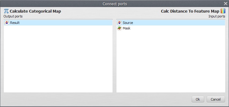
Now connect Categorical Map landuse.tif to Number Map, after setting the Map Number to “1”. Open Calc Distance to Feature Map with the Edit Functor Ports.
Source is a map containing the features to which distances will be calculated. A feature is represented by a non-null value. Mask is a map used to mask the distance calculation on its null cells. Let’s connect the output from Calculate Categorical Map to Source and Categorical Map landuse.tif to Mask. Now open the Calculate Categorical Map and write the following equation:
if i1 = 5 then 1 else null
Remember that 5 is the number identifier for urban. You do not need to change either Cell type or Null Value in both functors, although to save memory you could set “Signed 8 Bit Integer” and Null Value to “0” in Calculate Categorical Map. You may also turn on the option Truncate Distance in Calc Distance to Feature Map. This will avoid exceeding the maximum numerical representation selected for Cell type.
Now connect the port Distance in Calc Distance to Feature Map to Save Map. The model should be ready to run. Always save the model before putting it to run. Save it as my_MCE_part1&2.egoml. Examine the result with the Map Viewer.
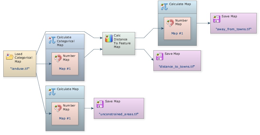
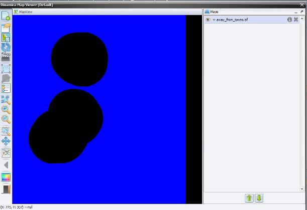
As a last procedure, add one Calculate Map and its Number Map, connect the output of Calc Distance to Feature Map to its Number Map and output the result with Save Map away_from_towns.tif. Notice that at this stage, we are omitting some steps, which should be well-known by now. Write in the equation box of the Calculate Map:
if i1 < 10000 then null else 1
You will have the following model.
Save and run it. Open the map away_from_towns.tif. Is this what you got?
How would you solve the problem having the following criteria?
- Distance to major roads < 15 kilometers.
- At least 1000 meters away from flooded plains.
You will need to load another Load Categorical Map and enter the file mainroads.tif from folder lesson5. You will need to turn on the option Define Null Value and set the Null Value to “0”. You can connect this functor directly to another Calc Distance to Feature Map that you will need to place on the sketch. Use Categorical Map landuse.tif again as the Mask.
Use the following equations in the respective Calculate Map (you will need to place one for each criterion):
if i1 > 15000 then null else 1
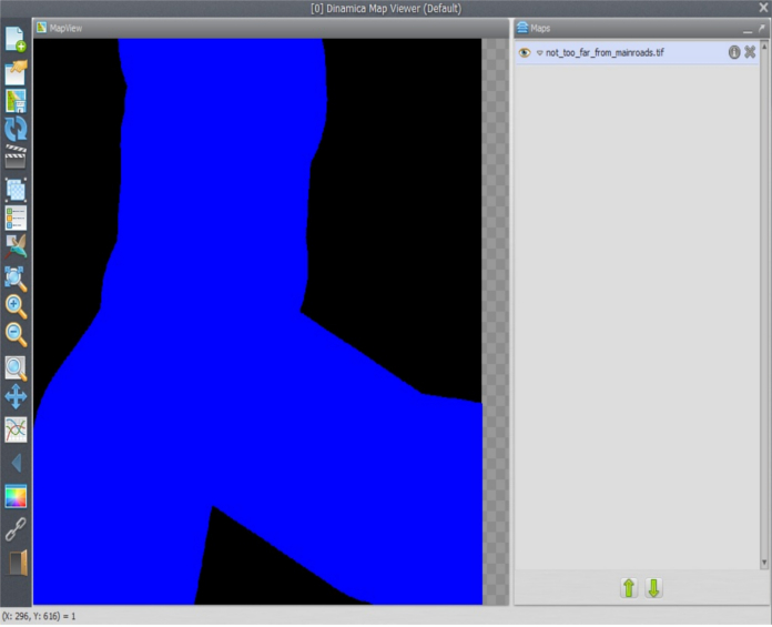
Now connect its output to Save Map not_too_far_from_mainroads.tif.
You will have the following model.
Check its integrity, save as my_MCE_part1&2.1.egoml and run it.
Did you get a not_too_far_from_mainroads.tif map like this?
For the flooded plains criterion, you will need to add another Calculate Categorical Map to pinpoint the flooded areas before passing the resulting map to Calc Distance to Feature Map.
Connect Categorical Map landuse.tif to it and write the following equation in the Calculate Categorical Map equation box:
if i1 = 0 then 1 else null
Now connect this output to Calc Distance to Feature Map as the Source port, again use Categorical Map landuse.tif as the Mask port, then connect its output to another Calculate Map and write the following equation:
if i1 < 1000 then null else 1
Save the output as malaria_free_zone.tif
The model for the three criteria combined should look like this:
Check the model, save it as my_MCE_part1&2complete.egoml, run and analyze the map malaria_free_zone.tif. Does it look like this?
Third step: Calculating driving time to neighboring towns
Driving traveling time to neighboring towns must not exceed 30 minutes. This fourth criterion requires the use of Calc Cost Map as well as a transportation friction surface.
To solve this criterion the model will establish two speeds of traveling: one for the road network and another for all types of land uses. Traveling on road has an average speed of 60km/h. Thus the corresponding speed to cross a unit cell of 100 meters of resolution will be 0.1 minutes. In turn, traveling through the outback has an average speed of 20 km/h, which is equivalent to 0.3 cell/minute.
Explanation x (hour) → 0.1 km 1 h → 60 km This is equal to = 0.1 km/60 km x 60 minutes = 0.1 minute
Let’s then reclassify Map landuse.tif to produce the friction surface. In order to this you need to place another Calculate Map and write into its equation box the following equation:
if i1 = 6 then 0.1 else 0.3
Now connect its output to a Calc Cost Map functor (to its Friction port). You will need another Calculate Map to pinpoint the neighboring towns from the land-use map using the equation below:
if i1 = 5 then 1 else null
After connecting the output of the last Calculate Map to the Calc Cost Map functor (to its Source port), pass the output of the Calc Cost Map to another Calculate Map to produce a Boolean map according to the maximum time of traveling, as follows:
if i1 < 30 then 1 else null
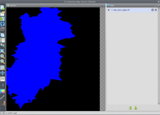
Finally save the output map as near_town_region.tif. Note that you have added to the model three additional Calculate Map functors, three Number Map functors, one Calc Cost Map and another Save Map. The model should look like the following figure.
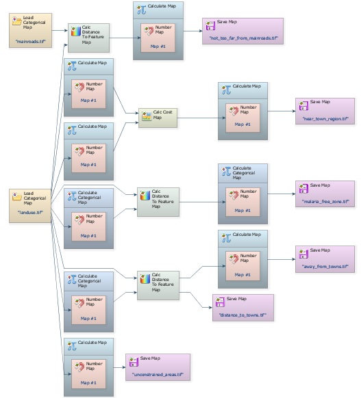
Save the model as my_MCE_part1&2&3.egoml, and run it. Examine map near_town_region.tif. Is this what you got?
Fourth step: Combining the Boolean criteria
So far you have solved the following criteria:
- Distance to main roads < 15 kilometers.
- Driving distance to neighboring towns < 30 minutes
- At least 10 km away from existing towns.
- At least 1000 meters away from flooded plains.
- In addition, we need to consider that not all land is available. We don’t want to encourage more deforestation in the region, thus using only land that is deforested or abandoned. Also existing urban areas, rivers and flooded plains must be excluded.
The two remaining criteria (areas equal or greater than 1000 hectares, and average slope < 0.5 degrees) must be solved using a zonal approach as provided by the Region functors. Before moving on to this step, you need to combine all criteria already solved into a single map.
As you have noticed this model has reached a certain level of complexity, and it beginning to become difficult to grasp its structure through the graphical interface. Dinamica EGO presents some facilities to reduce the visual complexity of models.
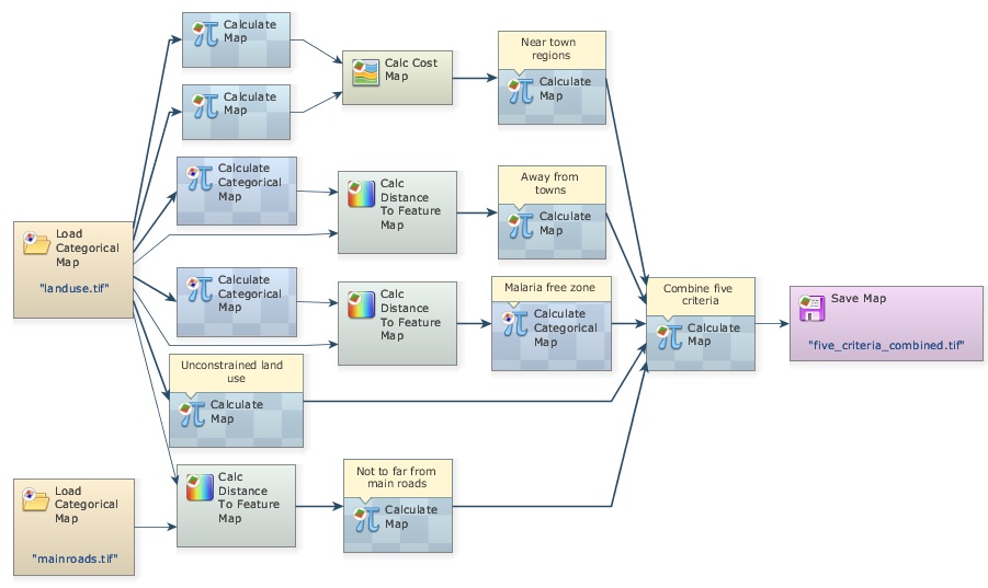
Firstly, you can delete the Save Map functors, since you have already checked their results. Second, you can add comments to some functors highlighting their outcomes. Let’s do it!
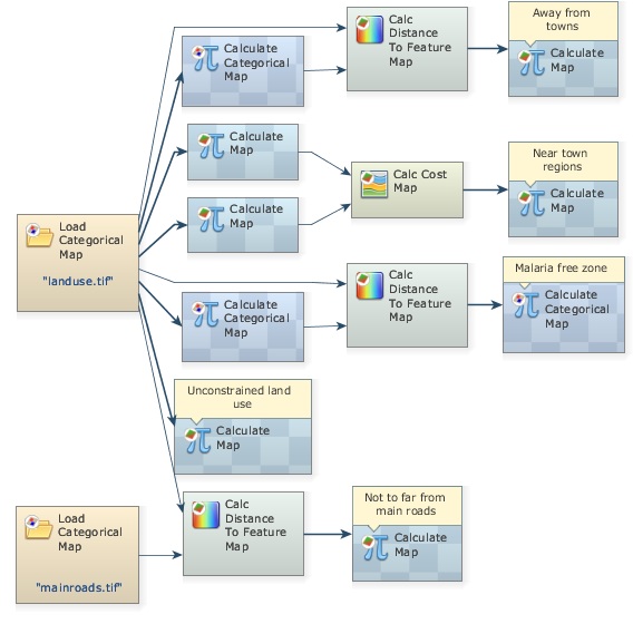
Grab the Add Comment to Functor tool from the sketch toolbar. Describe the outcome in each functor preceding the Save Map functors, so you can trace each data flow back to its initial node (that is Map landuse.tif). Do it by clicking on its top left icon.
Write in respective functors: Near town regions, Malaria free zone, Away from towns, Unconstrained land uses, Not too far from main roads.
At this stage, you can delete the Save Map functors, since you have already checked their results. After doing so, organize the layout from left to right.
The five titled Calculate Map functors produce the five criteria solved so far. Now you just need to combine them with Calculate Map.
Now place five Number Map functors within it. Open it and write the following equation.
i1*i2*i3*i4*i5
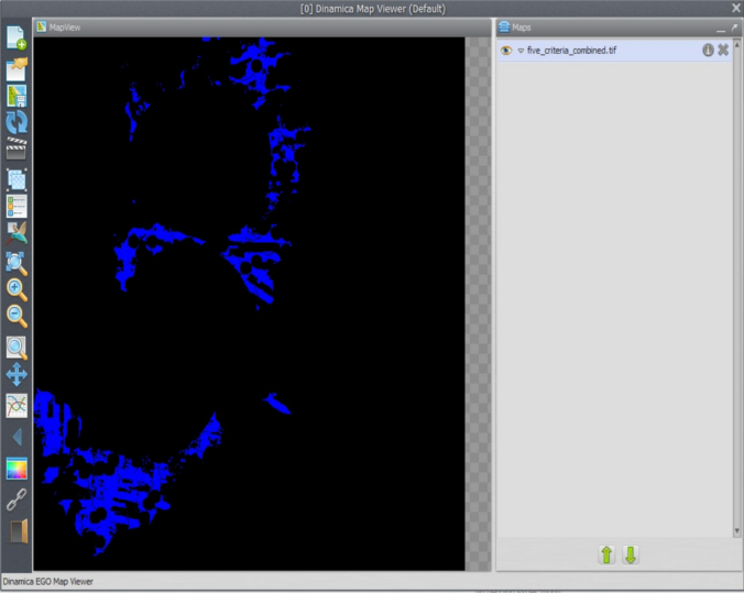
Change Cell Type to “UnSigned 8 Bit Integer” Null Value to “0”; write the comment “Combine five criteria” and add Save Map to view the result, naming the file as five_criteria_combined.tif. Finally organize the layout left to right.
Close the right-most container to show the comments, save the model as my_MCE_part1&2&3&4.egoml, check and run it. Is this what you get?
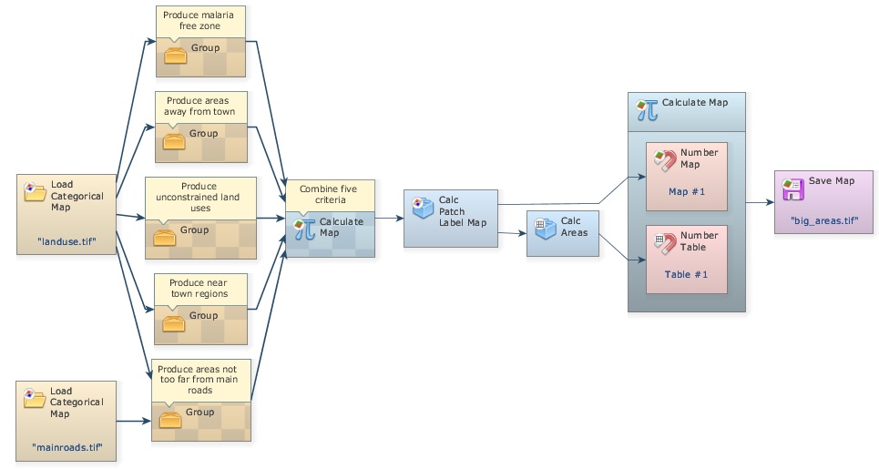
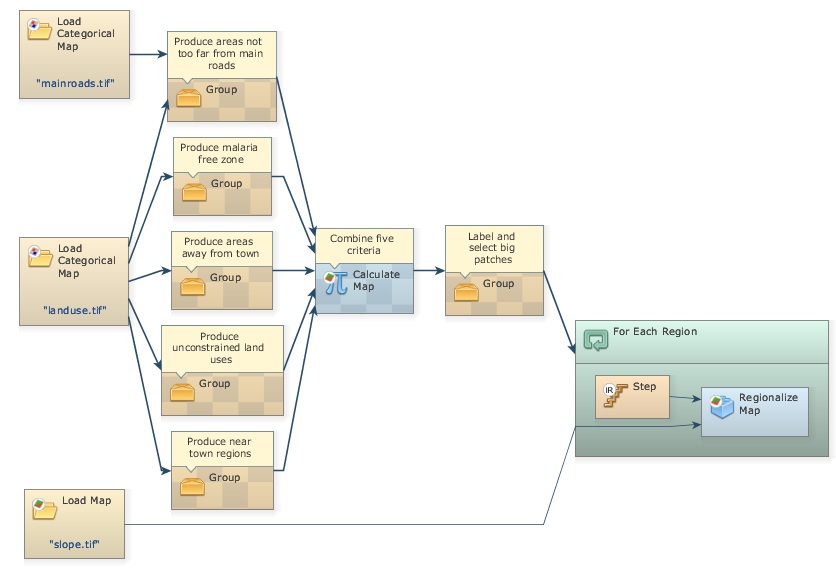
To further simplifier the view of the model, another resource available in Dinamica EGO is the Group functor. Drag five Group functors from the Control tab and place them on the sketch. Now select each functor of a data flow chain that ends up in Calculate Map “Combine five criteria” (Press Crt + right button to keep on continually selecting functors), leave the Categorical Map functors out, now drag them into a Group. Repeat this procedure for the five criteria.
Close each Group and write the following comments in their respective Group. You may need to zoom in.
Produce near town regions
Produce malaria free zone
Produce areas away from towns
Produce unconstrained land uses
Produce areas not too far from main roads
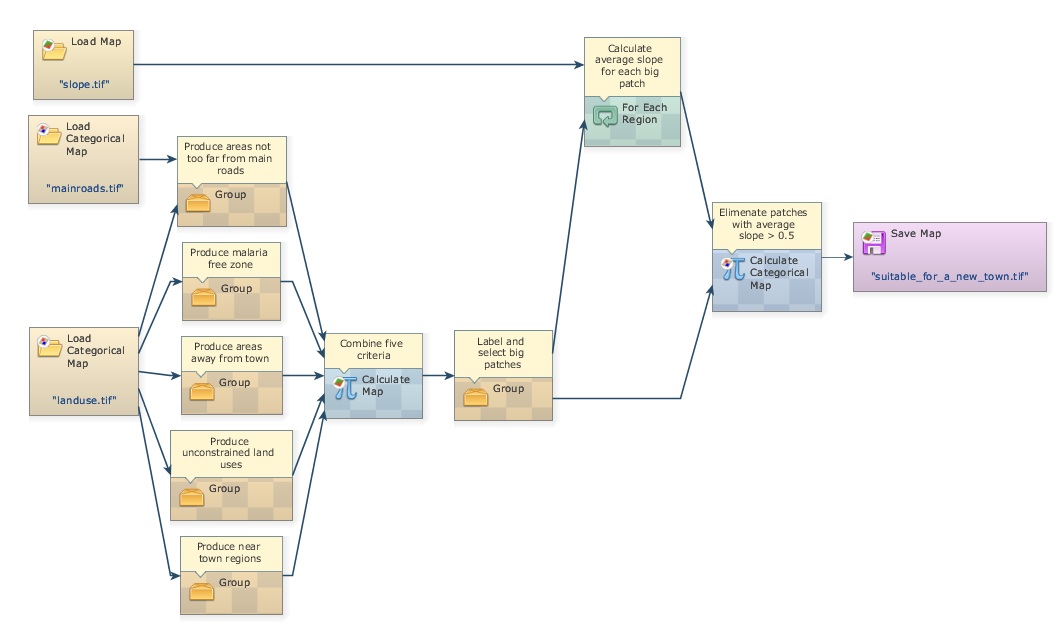
See model on the next page. Didn’t the model become much easier to visualize? Of course, you will need to open the Group functor to understand how the data are produced. You can do this one by one. Note that the function of the Group functor is to help organize the model diagram.
Save this model as my_MCE_part1&2&3&4group.egoml and let’s move forward to the next step.
Fifth step: identifying suitable areas
In this step, you will identify the suitable areas equal to or greater than 1000 hectares. First, delete Save Map five_criteria_combined.tif. Remember that the less the software accesses the disk, the faster the model runs. Now, drag from Map Algebra tab the functor Calc Patch Label Map. This functor labels patches of cells using sequential numbers. A patch consists of a continuous group of neighboring cells of the same category (see also Landscape metrics in Dinamica EGO). You need this in order to solve the area criterion. Connect the output from “Combine Five Criteria” to it. Some of its parameters are:
Initial Patch Label: Set it to “1”.
This will be sufficient to store all patch label number identifiers. Leave the other parameters untouched. Go to help for further details. Now connect its output to Calc Areas, available in the Map Algebra tab. As output this functor provides one table with three columns. See notes for additional information about the Calc Areas result.
Now, place on the sketch one Calculate Map and one Number Map and one Number Table within it. Connect Calc Areas to Table 1 (this implies that output of Calc Areas is a lookup table), and Map output from Calc Patch Label Map to Map #1. Now open Calculate Map and write:
if (t1[ [i1][“Area_In_Hectares”] ] < 1000) then null else 1
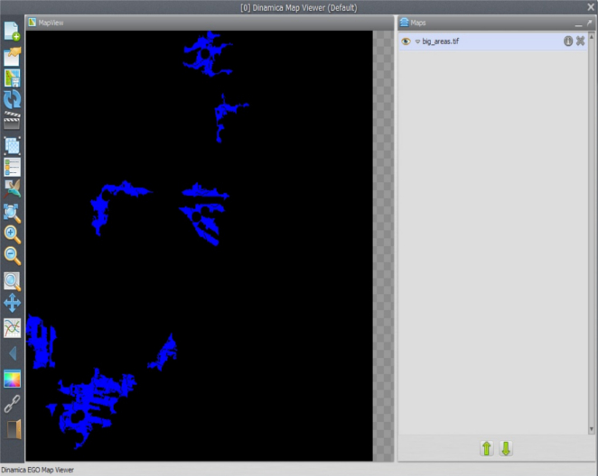
Using this formula, the functor will analyze the size of each patch and then eliminate the patches smaller than 1000 hectares. Now place one Save Map and enter big_areas.tif.
Check the model, save it as my_MCE_part1&2&3&4&5.egoml, run it and examine its output. Is this what you got?
Great, what a haul! But before moving on to the next step, there is still a last thing to do. In order to keep the patch labels, you need to multiply the output from the last Calculate Map, to which you have added the comment “Identify big patches”, with the output from Calc Patch Label Map. Therefore, you will keep only the labels for the big patches.
Place one Calculate Categorical Map and two Number Map functors within it. Set their Number Map functors to “1” and “2” respectively, and remove the Save Map functor. Now connect functors as follows:
Write: i1*i2, close the functor and insert the comment “Keep labels only for big patches”. Now you are ready to move on to the last step.
Sixth step: identifying suitable areas 2
The final criterion establishes that the average slope on the selected patches must be less than 0.5 degrees. Place Load Map and load it with \lesson4\originals\slope.tif. Now revise Lesson3, as you will to need to reapply the concept of region.
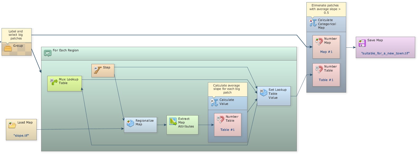
Drag For Each Region, Regionalize Map, and Step, insert the two latter functors within the previous and connect them as follows.
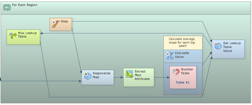
The map to be regionalized is the slope.tif. The map output from the last Calculate Categorical Map will control For Each Region. Remember that this functor enables the model to iterate according to the map categories passed to it. Now place one Mux Lookup Table, one Extract Map Attributes, one Calculate Value, one Number Table and one Set Lookup Table Value, all within For Each Region and connect them as follows.
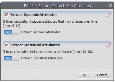
Write equation: t1[13] in the Calculate Value. Remember that 13 is the key for the average of all non null cells in the attribute table. This submodel is very similar to the one introduced in Lesson 3. Open Extract Map Attributes and set the option:
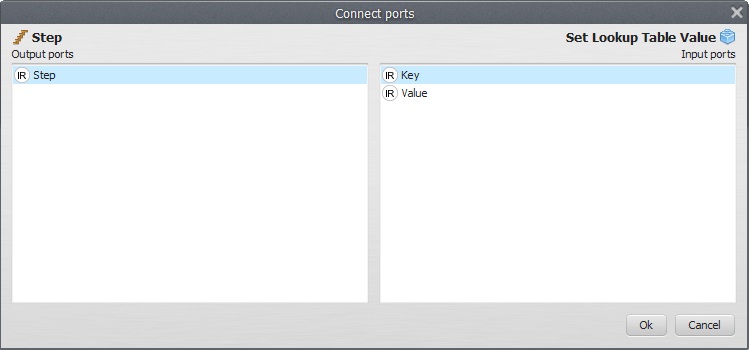
Remember to link Step to Key on the Set Lookup Table Value
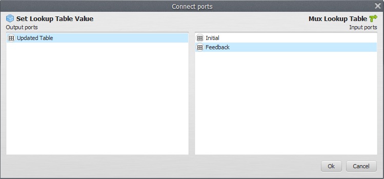
As well as Updated Table to Feedback
Open Mux Lookup Table with the Edit Functor Ports and click on Initial, enter a blank table. Just enter once “0” and “0”, as Key and Value. Register the Table output port to be viewed. You might want to see the results.
Finally place Calculate Categorical Map after the For Each Region and place Number Map and Number Table within it. Number them and write the following equation: if t1[i1] > 0.5 then null else i1
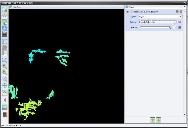
Save the result as suitable_for_a_new_town.tif on the lesson5 folder.
Check the model, save it as my_MCE_part1&2&3&4&5&6.egoml and run it. Is this what you got?
Finally you just need to organize the model in a more legible layout. Place one Group and drag Calc Patch Label Map, Calc Areas, Calculate Map “Identify big patches”, and Calculate Categorical Map “Keep labels only for big patches” into it.
Close it and add the comment “Label and select big patches”, close the Region Manager and add “Calculate average slope for each big patch”, close the last Calculate Map functor and add “Eliminate patches with average slope > 0.5” and lastly, add the comment “Save final map” to Map suitable_for_a_new_town.tif.
Save the model as my_MCE_part1&2&3&4&5&6_complete.egoml. This is the final model.
HOME WORK
Examining the map suitable_for_a_new_town.tif, you will note a large patch on its southwest portion, which would be the best target for a new town, considering the areal extent as an additional criterion. Would you be able to add a submodel to the current model to pinpoint this patch?
