Spatial Patterns of Changes
As Dinamica EGO was designed to be a general purpose dynamic modeling software, we present a collection of spatial patterns produced by the various combinations of its transition functions. In order to evaluate the wide range of Dinamicas’s possibilities, a series of simulation were run using synthetic simplified maps. The results for each model are presented as follows:
H0 to H8 are run, for a sole time step, by using a transition matrix 2×2 that models only one transition – from class 2 to 1 – with a rate of 0.01. The landscape map encompasses a matrix of 132 by 132 cells and all cells have equivalent spatial transition probability, which means that ancillary variables are not used to influence the cell allocation process.
| H0 |  | There is no spatial arrangement and no patch aggregation. The allocation process takes place randomly and does not interact with the neighborhood. The dynamics is only controlled by the transition matrix. |
| H1 |  | The allocation process is set to form patches with a patch mean size of five cells, patch variance is set to zero. Only the Patcher functor is used. The Patcher isometry factor is set to zero, which means that the patches tend to be most linear as possible. |
| H2 | 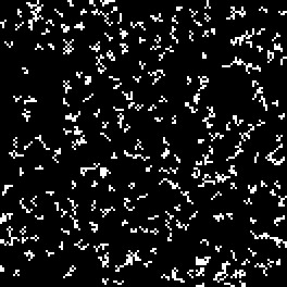 | The allocation process is set to form patches with a patch mean size of five cells, patch variance is set to zero. Only the Patcher functor is used. The Patcher isometry factor is set to 1, the patches still take linear form, though shorter. |
| H3 |  | The allocation process is set to form patches with a patch mean size of five cells, patch variance is set to zero. Only the Patcher functor is used. The Patcher isometry factor is set to 1.5, now the patches assume a more isometric form. |
| H4 | 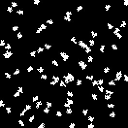 | The allocation process is set to form patches with a patch mean size of 20 cells, patch variance is set to zero. Only the Patcher functor is used. The Patcher isometry factor is set to 1.5. Notice the fewer and larger patches. |
| H5 |  | The allocation process is set to form patches with patch mean size of 200 cells, patch variance is set to zero. Only the Patcher functor is used. The Patcher isometry factor is set to 1.5. Only seven patches are formed. Patches tend to aggregate. |
| H6 |  | The allocation process is set to form patches with patch mean size of 20 cells, patch variance is set to 180. Only the Patcher functor is used. The Patcher isometry factor is set to 1.5. Path size varies greatly. |
| H7 |  | Only the Expander functor is used with patch mean size of 1742 cells, which is tantamount to the expected number of transitions. Patch variance is set to 0. The Expander isometry factor is set to 1.5. Notice the single patch produced around a cell of class 2 located at the center of the map. |
| H8 |  | The transition functions are used in a combination of 0.8 of Expander and 0.2 of Patcher. Patch mean size is set to 600 with patch variance of 0. The isometry factor is set to 1.5. Two more patches are produced around the expanded central cell. |
H9: Transitions occur as a function of the spatial probability. DINAMICA sets up a spatial transition probability map for each transition, based on the weights of evidence chosen for specific ranges of each spatial variable stored in the static cube raster dataset. Simulation is run in 15 steps, with a rate of 0.005 per step for transition 2-1. Only the Patcher functor is used with patch mean size of 20 and patch variance of 0. Patch isometry is equal to 2. As a result, patches tend to form around the center of the map. The figures bellow depict, respectively, the static variable map, the calculated spatial transition probability map, and the simulated landscape.
H10: Transitions occur as a function of dynamic spatial probability. DINAMICA calculates dynamic distances to cells in previous state 2 and uses it to set up a spatial transition probability map based on the weights of evidence chosen for specific ranges of distance. Since a dynamic distance map is used, a new transition map is calculated during each iteration. Simulation is run in 15 steps, with a rate of 0.005 per step for the transition 1 to 2. Only the Patcher functor is used with patch mean size of 20 and patch variance of 0. Patch isometry is equal to 2. As a result, patches tend to nucleate around previous patches. The figures bellow depict, respectively, the dynamic distance map, the dynamically calculated spatial transition probability map, and the simulated landscape.
To test its a ability in simulating multiple transitions, simulations from H11 to H15 are run for a transition matrix 6 by 6. See figure bellow.
H11: There is no spatial arrangement and no patch aggregation. Expander percentage is 0, patch mean size is 1, and patch variance is 0. Transitions take place randomly only obeying the amounts of change set by the transition matrix. Simulations are run for 10 time steps. The figures bellow depict, respectively, the original landscape map, and the simulated landscape.
H12: There is no spatial arrangement but patch aggregation. Patch mean size is set to 5, and simulation is run for 10 time steps.
H13: There is no spatial arrangement but patch expansion produced by the sole use of the Expander functor. Patch mean size is set to 1, and simulation is run for 10 time steps. The left figure depicts the result for patch isometry equal to 1 and the right figure for patch isometry equal to 1.2
H14: There is no patch aggregation but now each transition is influenced by its spatial probability map computed over maps stored in the static raster cube. Expander percentage is 0, patch mean size is 1, and patch variance is 0. Simulations are run for 10 time steps.
Figures bellow in B&W represent the Weights of Evidence function, respectively, for transitions 1-2, 1-3, 1-4, 1-5, 1-6. The color figure represents the transition probability map for 1-2 computed by integrating the single Weights of Evidence functions. The last two color figures depict the simulated landscape maps after 1 and 10 iterations.
In conclusion, the combination of Dinamica’s transition function presents numerous possibilities with respect to the generation and evolvement of spatial patterns of change. As a result, Dinamica can be considered as a potential tool for the replication of dynamic landscape structures. The calibration of a simulated landscape can be achieved by a series of simulation using varying parameters. An approximated solution can be attained comparing landscape metrics, such as fractal index and mean patch size of the simulated maps with the ones of the reference landscape. We intend to incorporate in the next version of Dinamica an automatic calibration procedure aiming at the match of spatial patterns.
