New Road Constructor

• This page describes the submodels and algorithms used as foundations for defining a new road constructor for use with Dinamica EGO LUCC models.

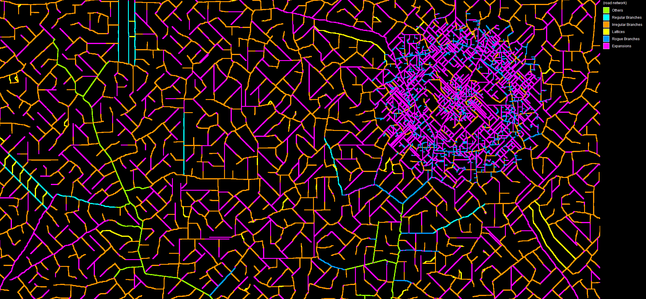
                                                               Examples of road network constructed using the tools described below

Roads used by the new road constructor tool are always adapted by a process we call “canonization”. The cells in their canonical feature representation are always connected using a Von Neumann neighborhood (https://en.wikipedia.org/wiki/Von_Neumann_neighborhood, cross pattern). This representation has the advantage of turning features into barriers, preventing them from being “crossed” by cost surface calculations (this restriction is important for all algorithms described below). The canonization can optionally bridge one-cell wide gaps that might be splitting some of the input features in separate features. The canonization process is automatically applied by any of the road construction algorithms.

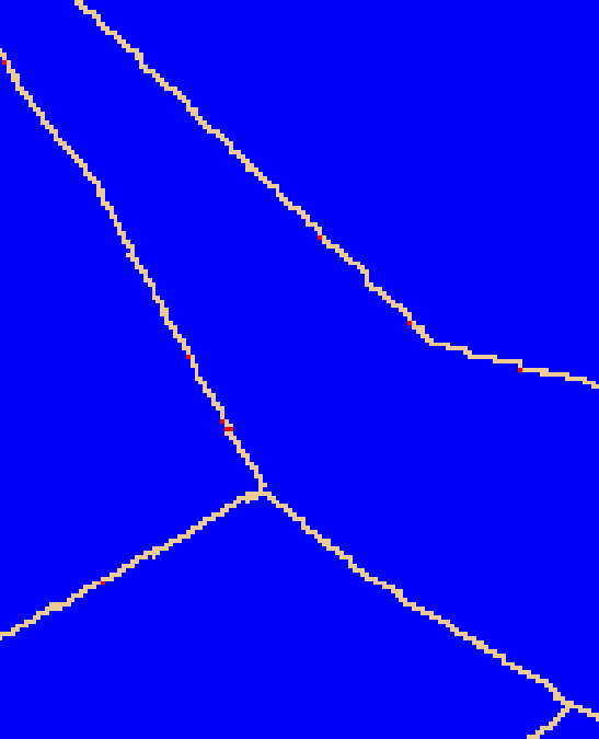
                                 Example of a road in modified to be in its canonical form - red cells represent areas modified during the canonization procedure

The road constructor is formed by a combination of one or more of the following submodels:

• Build Road Expansions
• Build Irregular Branches
• Build Regular Branches
• Build Road Lattice

Existent roads are expanded by sprouting new segment from their endpoints.

1. First, it calculates a map depicting only the cells representing the endpoints of the given features. Endpoints are detected using a technique described in the paper Convolution Approach for Feature Detection in Topological Skeletons Obtained from Vascular Patterns (psu.edu). Each endpoint is assigned a unique id value. Optionally, branches in features that are only one-cell long can be ignored. The feature map must be provided in their canonical representation.

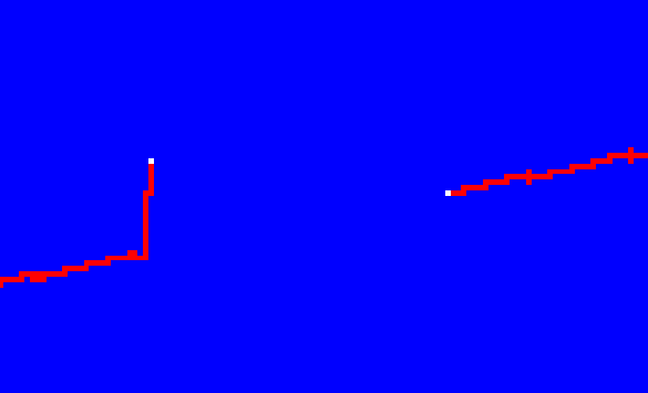(example of road endpoints – white cells represent the areas depicting the road endpoints, but ignoring branches that are only one cell long)

2. Then, it calculates the cost and direction map to reach the “least costly” road endpoint. The existent roads are treated as barriers which can make some parts of the map inaccessible to the cost calculation.

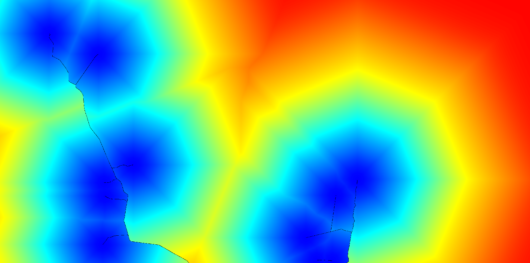(costs to reach the “least costly” road endpoints –“blueish” areas represent the vicinities of road endpoints)

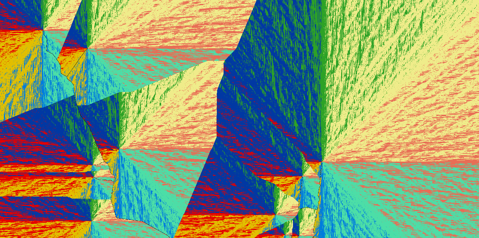
(directions that must be followed to reach the “least costly” road endpoints)

3. As the next step, the resulting cost map is used to group the reachable cells using an allocation calculation. This process defines which endpoint dominates each area of the map. Additionally, the dominance areas are “fenced” preventing any following cost map calculations from crossing the area boundaries.

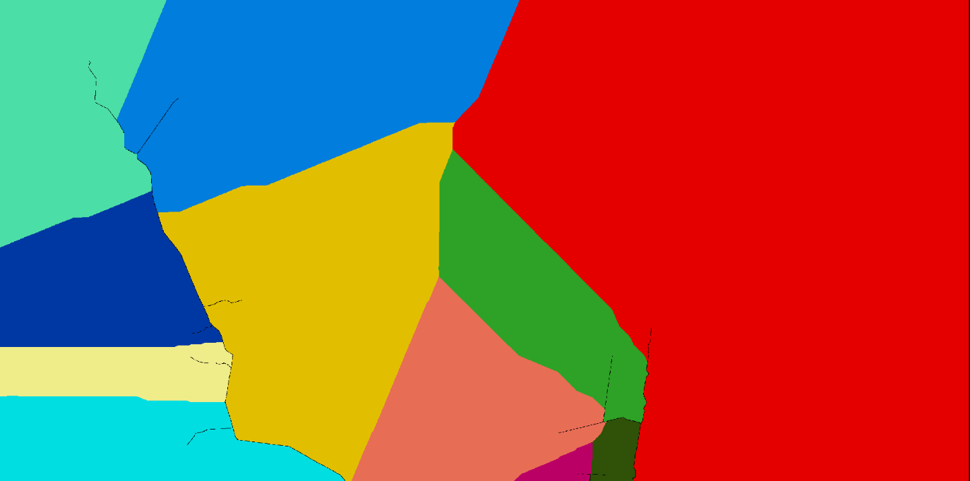(road endpoint dominance areas – each color corresponds to the region of dominance of a road endpoint located in that area)

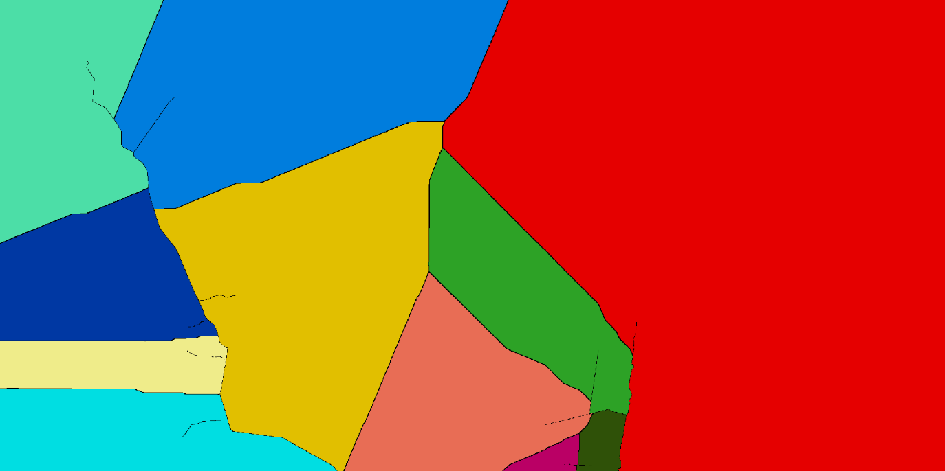(road endpoint dominance areas with “fences” around them – “fences” are made of contiguous null value cells)

4. Now, for each endpoint dominance area, it calculates the angle (in degrees) between all cells and the corresponding feature endpoint vector. The calculation uses theta = acos(dot(u, v) / (mod(u)*mod(v))), where u is the vector representing the feature endpoint direction (which is also calculated for each of the endpoints, using the same technique described in the paper Convolution Approach for Feature Detection in Topological Skeletons Obtained from Vascular Patterns (psu.edu)) and “v” is the vector representing the direction of the new possible feature segment. The direction of each one of the endpoints is a discrete value and uses one the following eight possible representations: NW=1, N=2, NE=3, E=4, SE=5, S=6, SW=7, W=8 and Undefined=0.

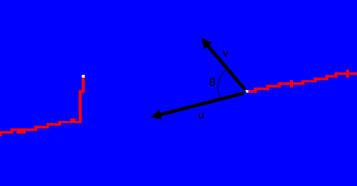(calculation of road endpoint angles)

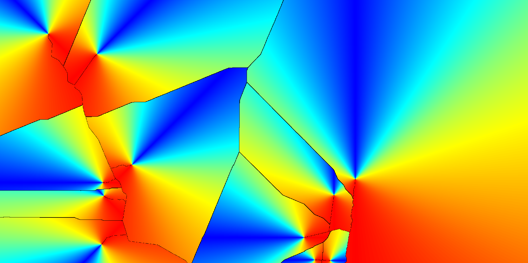(angle map – blueish values represent small angles while red values represent large angles)

5. The resulting angle map is then filtered: angles and “areas” satisfying a set of constraints, such as “Maximum Road Travel Cost “and “Maximum Road Ending Vector Angle”, are used to define a “viable” cone-shaped area per road endpoint in the friction map. This friction map will be used to calculate another cost map in the next step. The “Minimum Road Travel Cost” is not used yet to ensure that cost calculations using the resulting friction map can still reach the corresponding road endpoint.

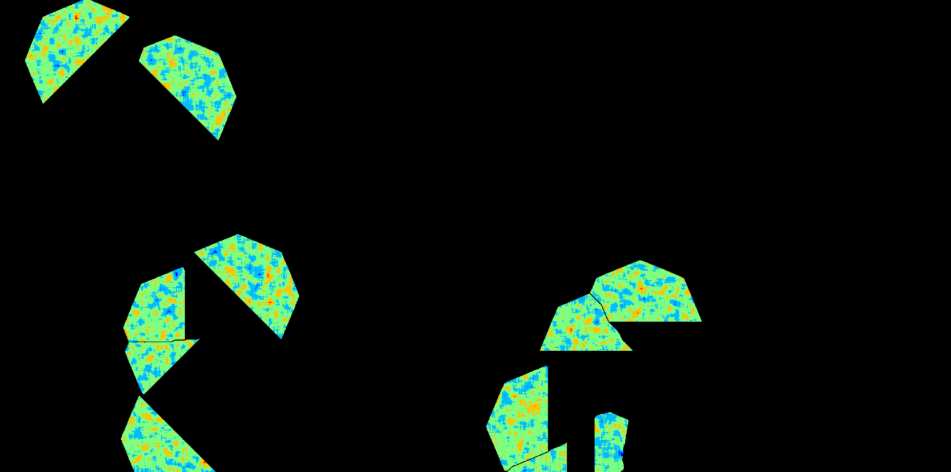(frictions within the “viable” cone-shaped areas)

6. Now, it calculates the cost and direction map to reach the corresponding road endpoint within each cone-shaped area.

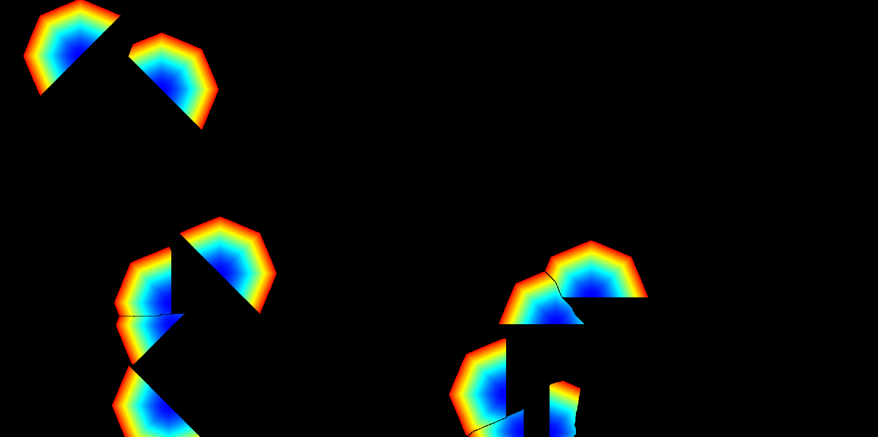(costs to reach the “least costly” road endpoints within the cone-shaped areas –“blueish” areas represent the vicinities of road endpoints)

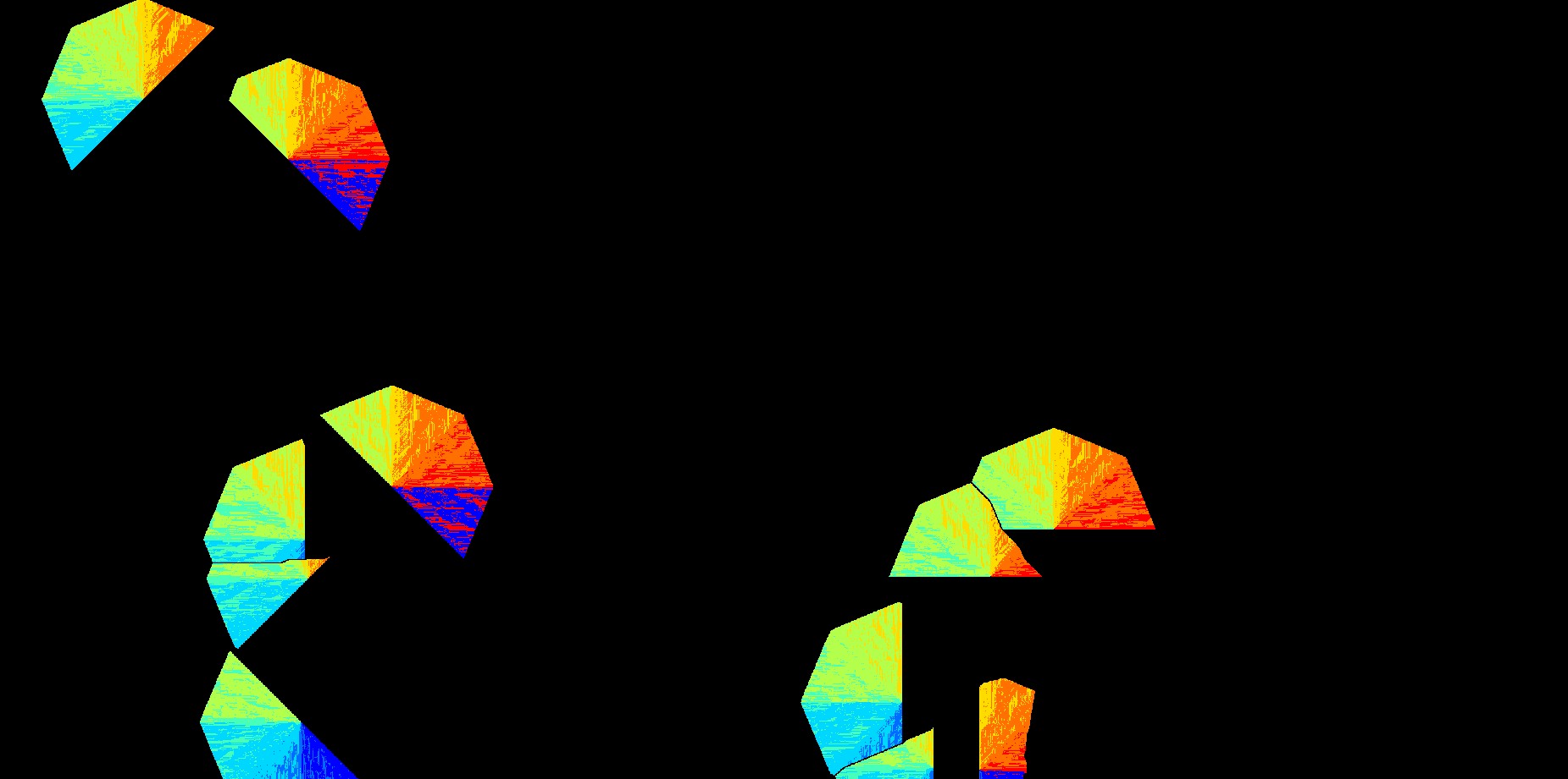(directions that must be followed to reach the “least costly” road endpoints)

7. Then, the cost map calculated using the cone-shaped areas, and the “Minimum Road Travel Cost” are used to filter the probability areas from where the new road destinations can be selected.

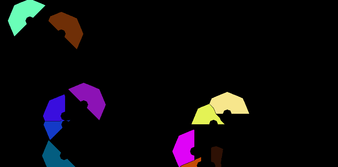(valid areas from where road destinations can be selected)

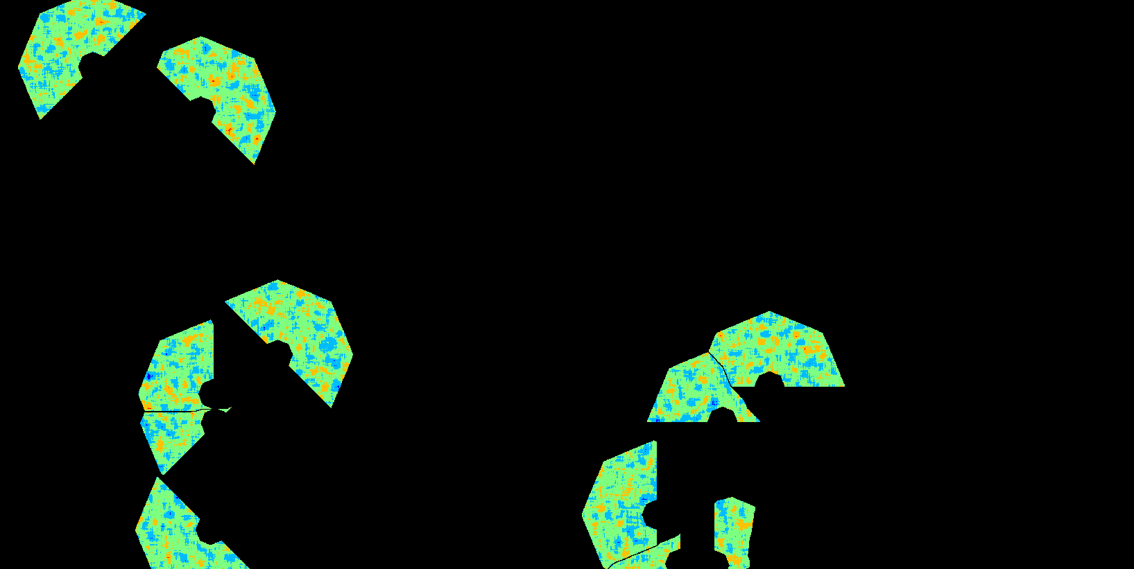(valid probabilities to select new road destinations)

8. As the last step, the selected new road destinations, together with the direction map, are used to construct segments connecting them and the corresponding road endpoint in their respective cone-shaped dominance area.

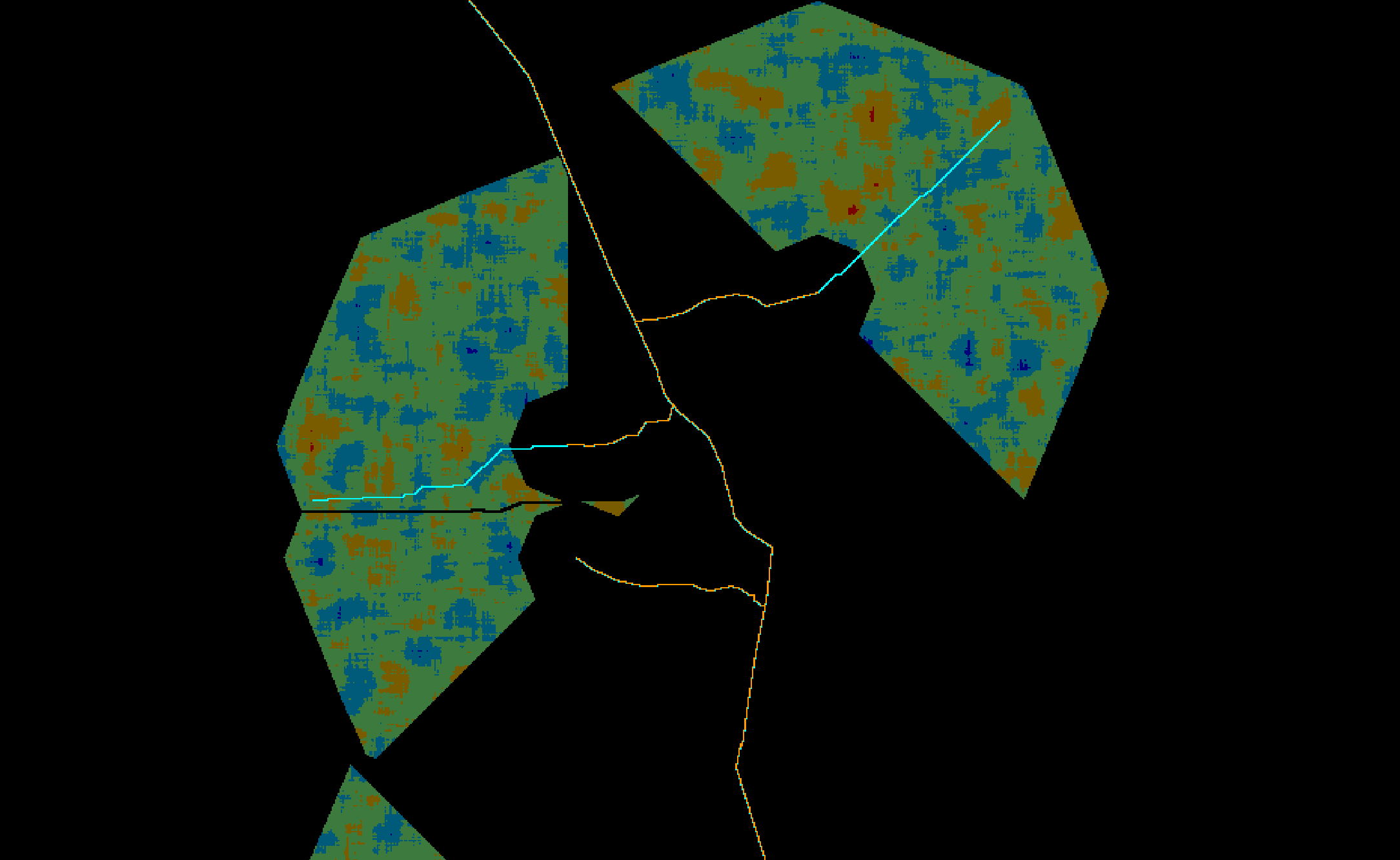(example showing some of the new road segments [cyan color] with the probabilities in their cone-shaped dominance areas in the background – the example shows only a portion of the previous images for better visualization)