This is an old revision of the document!
LESSON 18: Building a land-use and land-cover change simulation model
What will you learn?
* How to simulate land-use change
* How to calculate transition matrix
* How to calibrate a land-use change model
* Using Weights of Evidence
* Map Correlation
* Model Validation
This lesson explores the use of Dinamica EGO as a simulation platform for land-use and cover change (LUCC) models. The eventual goal is to calibrate, validate, and run a LUCC model for the Rondonia State in Amazon Biome, Brazil. Over the coming weeks you will learn how to calculate the amount of change using transition matrices, generate a probability map to help predict the locations of change, combine these two types of information within a model that propagates land change, validate your model based on observed changes, and then use the calibrated and validated model to project change into the future under various scenarios.
Step 1: Calculating Transition Matrices
The first step in building a land change model is determining the quantity of change. To do this, you will calculate historical transition rates. Transition rates represent the amount of each land cover class that is converted to every other land cover class over a specified period. In Dinamica, transition rates can be represented as real quantities of change (number of pixels or hectares) or as relative quantities of change (the proportion of the total pixels in a class that is converted to another class). Here, we are using relative quantities of change. These transition rates will later be passed to the LUCC model.
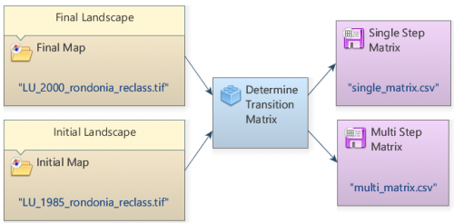
First, create an empty model to calculate transition rates, and save it. Then, build the model as depicted:

Connect Load Categorical Map LU_1985_rondonia_reclass.tif to the Initial Landscape port and connect LU_2000_rondonia_reclass.tif to the Final Landscape port.
Determine Transition Matrix can produce two different types of matrices. The single-step output corresponds to a period represented as a single time step. The multiple-step output corresponds to a time step unit (year, month, day, etc.). Like interest rates, transition rates are superimposed again and again over the stock variable, rather than simply being divided by the number of time steps. Double click on Determine Transition Matrix to define the number of time steps, which is 2000 – 1985 = 15 years.
Run the model!
Open the resulting matrices. Is this what you got?
Single Matrix:

Multi Matrix:

1. What percent of the total 1985 landscape is covered by each class?
2. What percentage of all lands on Oahu transitioned from one land use to another from 1985-2000?
3. What was the single biggest 1985-2000 transition in terms of total area? What was the total change in terms of hectares?
4. What was the smallest transition in terms of relative change? What was the annual rate of change for this transition from 1985 to 2000?
Step 2: Calculating Weights of evidence ranges and coefficients
Step 3: Weights of evidence correlation
Step 4: Calibrating Patcher and Expander
To calibrate the model, we will use the 2005 map as the initial landscape and the 2011 map as the final map. The landscape maps are signed 8-bit integer and represent the classes shown in Table 1.
Step 5: Generating Probabilities map and simulating LUCC
Step 6: Validating with exponential decay function and multi window similarity
Step 7: Projecting changes into the future (Trajetories)
Lesson under construction
Congratulations, you have successfully completed this lesson! Now let’s move to the next lesson: LESSON 19: The wizard editor in Dinamica EGO
